![]()
To deny our impulses is to deny the very thing that makes us human.
![]()
To deny our impulses is to deny the very thing that makes us human.
 |
HOWTO /
VarianceIn this tutorial, we will review how to use the energy variance as a measure of convergence of an MPS algorithm to some groundstate. This could be DMRG, or imaginary time evolution, or some other procedure. For demonstration purposes, we will use iDMRG with the spin-1/2 Heisenberg model. Some theoryWe can regard an MPS with finite bond dimension {$m$}, {$\vert \psi_0 \rangle$} as a perturbation of some exact state {$\vert \psi \rangle$} such that the energy per site of {$\vert \psi_0\rangle$} is {$E_0/L = (E + \epsilon)/L$}. As we increase the bond dimension of the MPS, then the difference {$\epsilon$} between the exact energy {$E$} and the variational energy {$E_0$} should decrease to zero. If we want to determine accurately the true groundstate energy {$E$}, we could attempt to extrapolate the variational energy {$E_0$} to the limit of infinite bond dimension. This is difficult to do directly with respect to the bond dimension; it requires obtaining a wavefunction that is well-converged with respect to the bond dimension (so the single-site density matrix mixing procedure doesn't work well, and requires reducing the mixing factor to 0), and in general the functional dependence between {$\epsilon$} and bond dimension {$m$} is not known. In the early days of DMRG, it was noticed that the truncation error, i.e. the discarded weight of the density matrix, is a suitable parameter to use for this extrapolation, because it scales linearly (or nearly linearly) with {$\epsilon$}. The DMRG codes in the Toolkit display the truncation error during the calculation, as a guide to the convergence as the program runs. However it doesn't display a truncation error at the end of the calculation, because there is another quantity that works better in almost all cases, which is the energy variance. The energy is an extensive quantity. From the theory of distributions (which also appears in thermodynamics), the variance of an extensive quantity is itself extensive. That is, the expectation value of the Hamiltonian evaluated on a system size of {$L$} sites is {$\langle \psi_0 \vert H \vert \psi_0 \rangle = E_0 L$}, where {$E_0$} is the energy per site. And likewise the variance is {$\langle \psi_0 \vert H^2 - E^2 \vert \psi_0 \rangle = \sigma^2 L$}, where {$\sigma^2$} is the energy variance, and {$E = E_0 L$} is the total energy. Given the MPO representation of H, finding the MPO for H^2 is just a matter of constructing the direct product of the MPO. We don't need to go to the bother of subtracting the energy, since we can evaluate the expectation value of {$H^2$} directly: {$$ \langle \psi_0 \vert H^2 \vert \psi_0 \rangle = E_0^2 L^2 + \sigma^2 L $$} So we see that the expectation value of {$H^2$} is a 2nd degree polynomial in the system size {$L$}; the prefactor of the {$L^2$} term is the square of the energy per site, and the prefactor of the {$L$} term is the variance per site. It appears to be a universal statement that the variance per site {$\sigma^2$} scales linearly with the error in the variational energy per site {$\epsilon$}, although I don't know of any rigorous proof of this in general. For a finite MPS with open boundary conditions, the behavior isn't strictly linear. This is because the local energy density near the open boundaries converges more rapidly than the local energy density of the bulk. Variance scalingIn a practical calculation, we can make use of the linear relationship between the variance and the error in the variational energy by plotting {$E_0$} as a function of {$\sigma^2$}, for a sequence of calculations with different bond dimension. In this example script, we will calculate the groundstate of a spin-1/2 Heisenberg chain using m=200 states, and then progressively reduce the basis size, constructing a sequence of wavefunctions with different bond dimensions. We will ultimately end up with wavefunctions
spinchain-u1 -o lattice
mp-idmrg-s3e -H lattice:H_J1 -w psi -m 10..200x1000 --create -u 2 -q 0
for m in 200 180 160 140 120 100 ; do
   mp-idmrg-s3e -H lattice:H_J1 -w psi -m ${m}x1000
   cp psi psi-m${m}
done
We can calculate the variance of these states using $ mp-imoments --power 2 -u 1 psi-m200 #mp-imoments --power 2 -u 1 psi-m200 #Date: Sun, 04 Sep 2020 19:38:50 +1000 #operator lattice:H_J1 #quantities are calculated per unit cell size of 1 site #moment #degree #real #imag #magnitude #argument(deg) 1 1 -0.44314701586468 5.1005315838889e-17 0.44314701586468 180 2 1 1.3774796042698e-07 -1.0853916472359e-18 1.3774796042698e-07 -4.514648370299e-10 2 2 0.19637927766977 7.722574447975e-18 0.19637927766977 2.2531446703282e-15 We added the For scripting purposes, we can do better than the output above. The energy and the variance correspond to the first two cumulants, so we can calculate the cumulants rather than the moments. We also only care about the real part of the output. Finally we don't need the header information at the top. Putting all these together, we can get some output in a much more scriptable format using $ mp-imoments --power 2 -u 1 --cumulants --real --quiet psi-m200 1 -0.44314701586468 2 1.3774796042698e-07 It is still slightly inconvenient in that we have the output split on two lines, and really we only need the second column. Some AWK magic can resolve this:
for m in 200 180 160 140 120 100 ; do
   mp-imoments --power 2 -u 1 --cumulants --real --quiet psi-m${m} | awk '{printf("%s ", $2)}'
   echo ${m}
done
This outputs 3 columns, the energy, variance, and basis size. If we direct this output to a file, say gnuplot> f(x) = a*x + E
fit f(x) 'output.dat' using 2:1 via a,E
set xrange [0:*]
set key left top
plot 'output.dat' using 2:1 title "iMPS data", f(x) title sprintf("Extrapolated energy %.10g", E)
This produces output similar to: 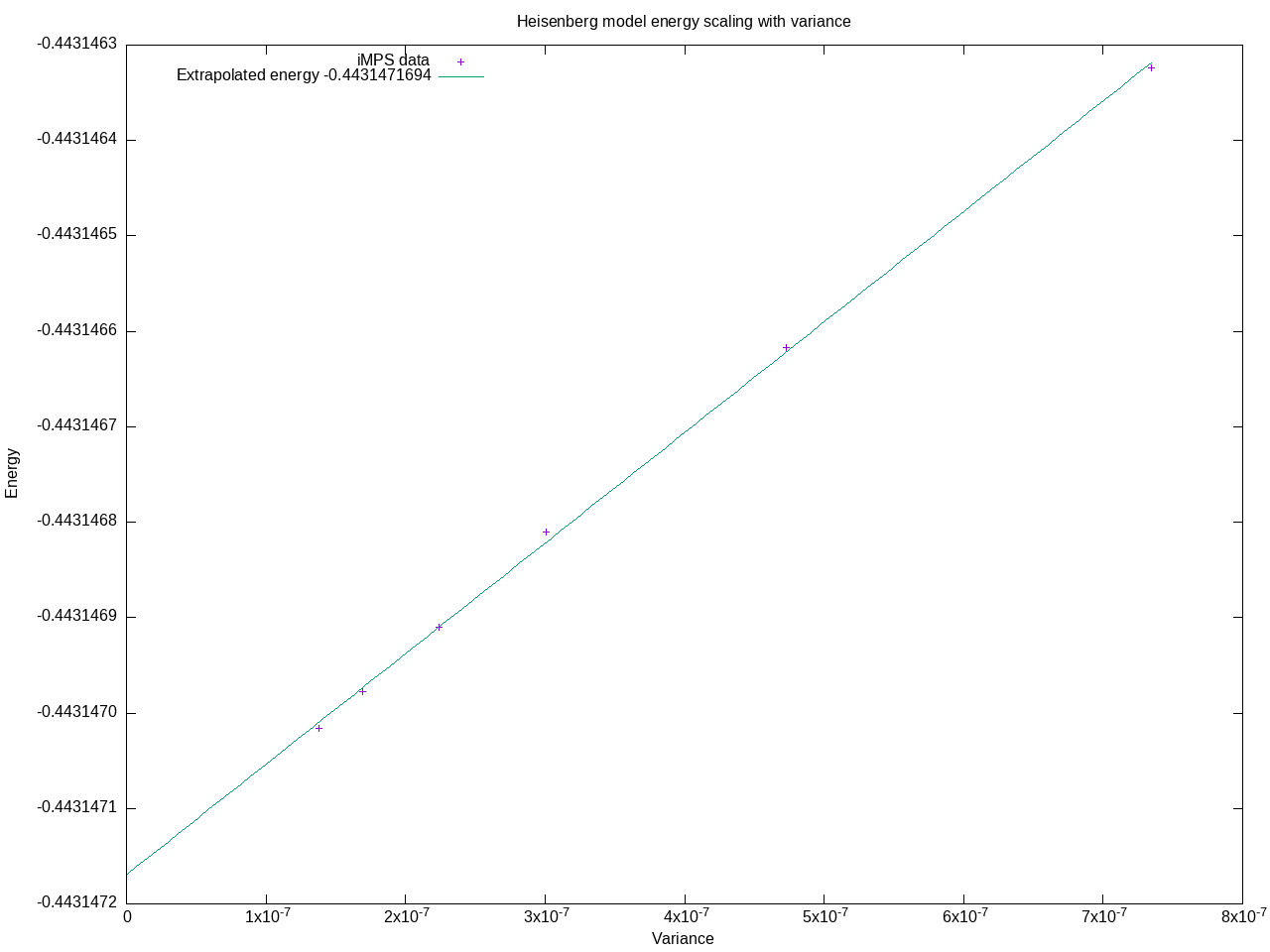 A useful refinement to this procedure would be to optimize the MPS further by scaling the density matrix mixing factor to 0 for each basis size. |