• View
• Edit
• Rename
• History
• Print
• Backlinks

TimeEvolution

In this tutorial, we will calculate the real-time evolution of a spin excitation in the S=1/2 Heisenberg model. In this tutorial we just calculate the local spin density in real space, but using this information it would be possible to construct a Fourier transform into energy/momentum space to construct the spectral function {$S(\omega, k)$}.

We will do this calculation for a finite size system. A better approach would be to use 'infinite boundaries'; that is, an excitation that exists as a finite window in the middle of a translationally invariant iMPS (see Phys. Rev. B 86, 245107 for details), however the ibc tools in the toolkit are currently experimental.

To construct a finite size state, we can re-use the lattice files and operators for an infinite system. So we start with a spinchain with {$U(1)$} symmetry,

spinchain-u1 -o lattice

Now to use finite-size DMRG we need an initial state. There are several ways to construct this initial state, but one of the simplest is to start from a random state.

mp-random -l lattice -u 100 -q 0 -o psi

This constructs a random state with 100 sites, with quantum number 0 (being the z-component of spin). We can now use this as input to the finite DMRG program, mp-dmrg.

mp-dmrg -w psi -H lattice:H_J1 -m 10..100x10,100x10
mp-dmrg -w psi -H lattice:H_J1 -m 100x10 --mix-factor 1e-4
mp-dmrg -w psi -H lattice:H_J1 -m 100x10 --mix-factor 1e-6

In this calculation, we started with a basis size of m=10 states, ramping up to 100 states over 10 sweeps. We then performed another 10 sweeps with the density matrix mixing factor reduced to 1e-4, and another 10 sweeps with mixing factor 1e-6. This produces a quite well converged wavefunction; we could keep going with smaller mixing factors and more sweeps but it won't change much in the wavefunction (increasing the basis size would have the single biggest effect on the accuracy).

We can now construct a local spin excitation, by acting on the wavefunction with an operator, for example {$S^+$} acting on the 50th site.

mp-apply lattice:"Sp(50)" psi psi-excitation

We can view the local spin density of the excitation using gnuplot:

gnuplot> plot '< for i in $(seq 0 99) ; do echo -n $i " " ; mp-expectation psi-excitation lattice:"Sz($i)" ; done' u 1:2 w lines title 'Spin excitation'

This produces output similar to: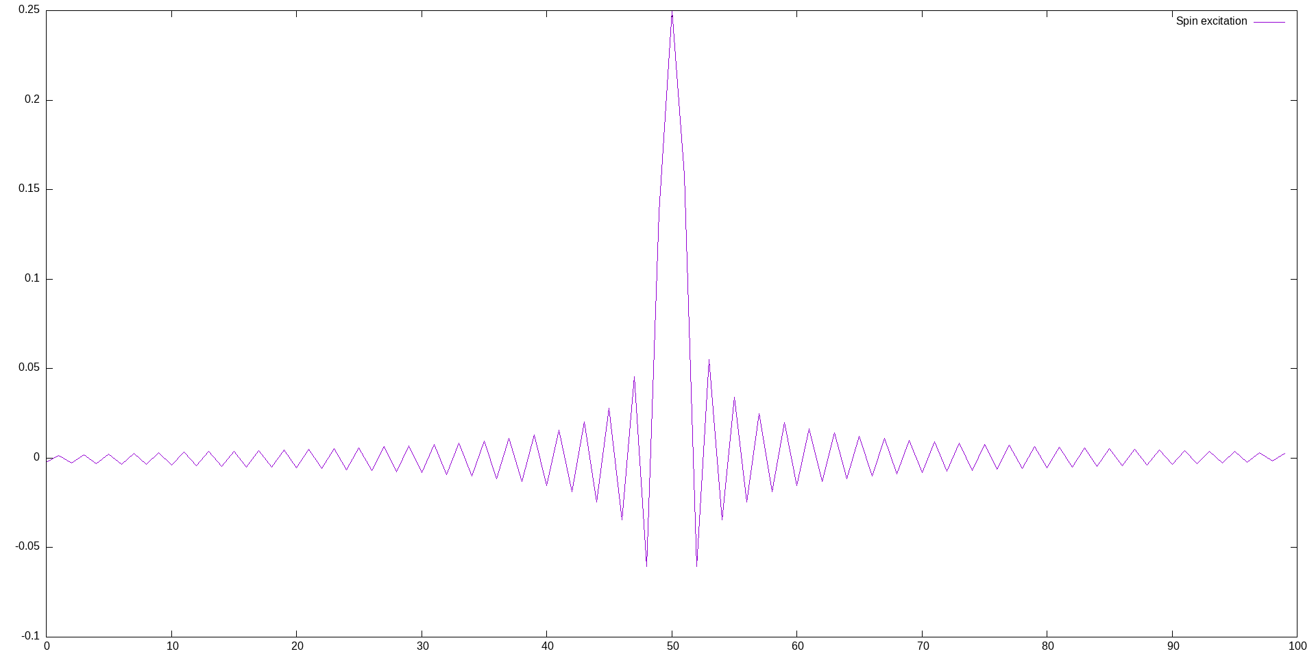

It is slightly asymmetric, because the open boundary conditions induces a slight odd/even dimerization, but this doesn't matter for our purposes.

Now we can evolve the state in real time using TEBD.

To see the various options of the mp-tebd program, run it without any parameters and you will get a list of all of the options, and a link to the online documentation. The parameters we need to use are:

mp-tebd -w psi-excitation -t 0.1 -s 1 -o psi-evolved -n 200 -m 100

The -w option specifies the initial wavefunction. The -t option is the timestep. The -s 1 option means save the wavefunction every timestep. If we only wanted to save the wavefunction every 10 timesteps, for example, we could use instead -s 10. The -o option is the output filename; the actual output file is this name followed by '.tXXX' where XXX is the timestep. If you don't supply -o then it uses the input filename. -n 200 means run 200 timesteps, and -m 100 limits the bind dimension to 100. In a real calculation we would want to use a larger bond dimension, or better still allow the bond dimension to grow by fixing the truncation error or setting a density matrix eigenvalue cutoff (for this calculation, a cutoff eigenvalue using the -d option of 1e-13 would work well).

We didn't specify the Hamiltonian here; this will default to the Hamiltonian used to construct the wavefunction, but if we wanted to specify a different Hamiltonian then we could supply one with the usual -H lattice:operator format.

This will take a few minutes to run (about 5 minutes, on my laptop), and will produce 200 wavefunctions, one for each timestep from 0.1 up to 20.0. Now we can calculate the local magnetization for each wavefunction. We could probably do this directly from Gnuplot, but it is annoying to have plot commands that take a long time to run, so we will save the data to a file using a bash script.

cp psi-excitation psi-evolved.t0.0
for t in $(seq 0.0 0.1 20.0) ; do ( for x in $(seq 0 99) ; do echo -n $x ' ' ; mp-expectation --real psi-evolved.t$t lattice:"Sz($x)" ; done > magnetization-t$t.dat ) ; done

Note that the first thing that we did was copy the t=0 initial state to the file psi-evolved.t0.0, so that we have a consistent naming scheme. Then our bash loop iterates over each file, writes a data file named magnetization.t[time].dat containing two columns, the site number, and the magnetization at that site. This also takes a few minutes to run, because mp-expectation isn't well optimized for finite lattices (this is a work in progress!).

Now we can plot the result using Gnuplot:

gnuplot> set xrange [20:80]
splot for [t=1:99] 'magnetization-t'.sprintf("%.1f",t/10.0).'.dat' u 1:(t):2:2:2 w lines palette lw 6 title ''

The output should look similar to: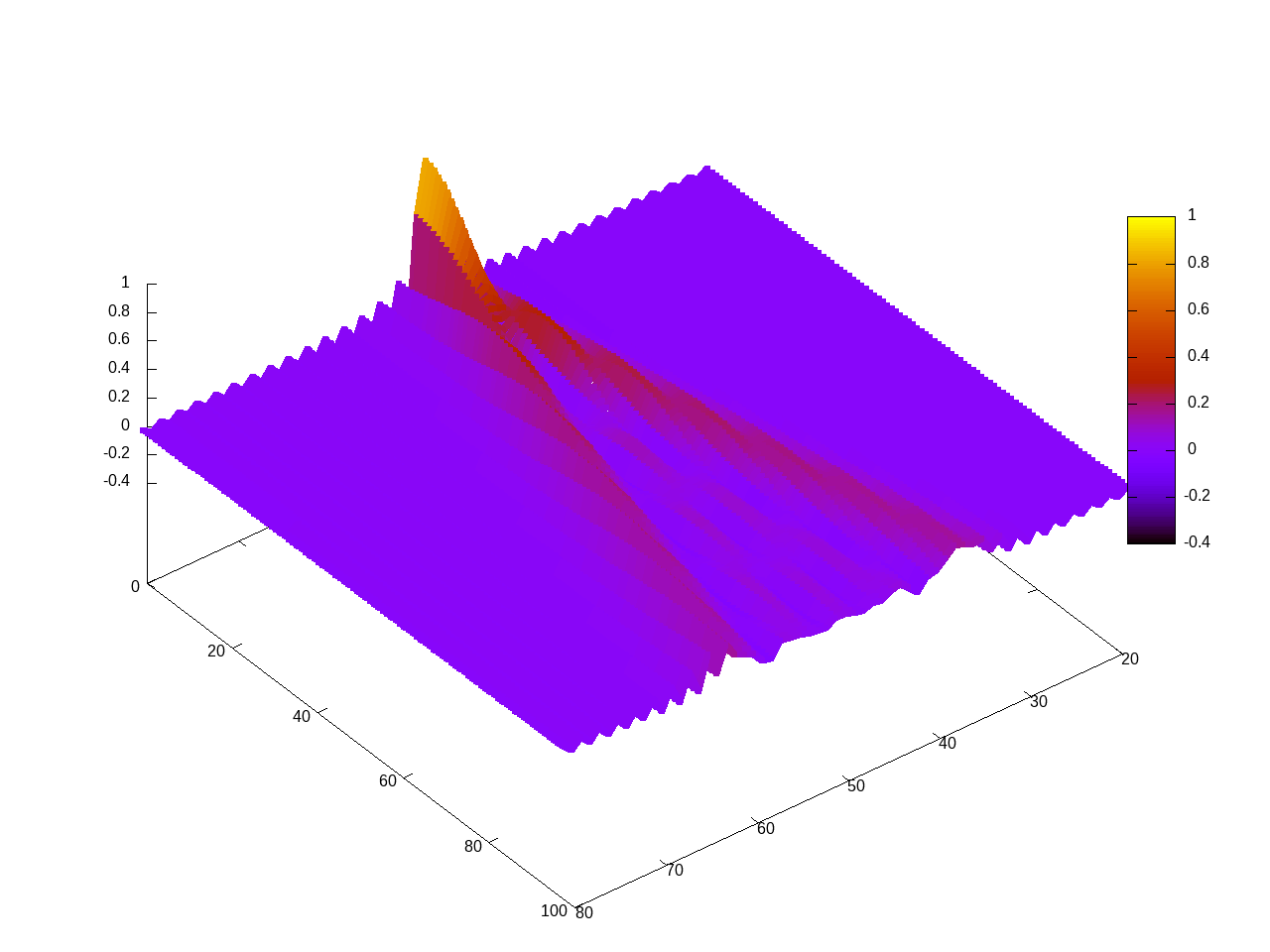