![]()
Throughout human history, we have been dependent on machines to survive. Fate, it seems, is not without a sense of irony.
![]()
Throughout human history, we have been dependent on machines to survive. Fate, it seems, is not without a sense of irony.
 |
HOWTO /
SingleModeApproximationIn this tutorial, we will use Matrix Product Operator techniques to obtain the excitation energy of a spin-chain using the Single-Mode Approximation (SMA). TheoryGiven the groundstate of some quantum system {$\vert \psi \rangle$}, we can construct a first-attempt Ansatz for an elementary excitation by applying some creation operator at a fixed momentum, for example for a spin chain we might attempt to construct the state {$$\vert k \rangle = S^+_k \vert \psi \rangle$$} For a non-interacting system, these are exact eigenstates of particle excitations. For an interacting system they will no longer be exact, but in some cases they can be a good approximation. One case where this approximation works reasonably well is the single-magnon excitations of the gapped S=1 chain. For an infinite system, we cannot construct the states {$\vert k \rangle$} directly as a standard iMPS. This is because they are not normalizable in the usual way. One way of seeing this is via the MPO representation of {$S^+_k$}, which has the form {$$W_{S^+_k} = \left( \begin{array}{cc} e^{ik} & S^+ \\ & I \\ \end{array} \right)$$} If we act with this MPO on an iMPS, we will obtain an MPS of twice the bond dimension, of the form {$$ \left( \begin{array}{cc} e^{ik} A^s & B^s \\ & A^s \\ \end{array} \right)$$} where {$B^s = \sum_{s'} \langle s \vert S^+ \vert s' \rangle A^{s'}$}. The resulting transfer matrix is upper-triangular and has a Jordan-block structure, so it isn't diagonalizable, hence it isn't normalizable in the usual way. In fact, the above state is an example of the excitation Ansatz, which is a distinct class of MPS. Another way of seeing this is to consider the norm of the state {$\vert k \rangle$}. The norm is given by the groundstate expectation value of the operator {$S^-_k S^+_k$}, which will be linearly extensive (for {$k=0$} it could be quadratic, but only for a magnetic state that has {$\langle S^+(x) \rangle \neq 0$}). Nevertheless, we can evaluate these expectation values using MPO techniques, which will be, in general, polynomials of the system size. The relevant expectation value that we want to calculate is the energy of the state {$\vert k \rangle$}, which is given by {$$ E = \frac{ \langle S^-_k H S^+_k \rangle } { \langle S^-_k S^+_k \rangle} $$} In this expression, the numerator will be a quadratic polynomial, so of the form {$ E L^2 + \Delta L$}, for some values of {$E$}, {$\Delta$} (the reason for choosing these names will become obvious shortly), and the denominator will be a linear polynomial, of the form {$ cL$}, for some value {$c$}. Thus the expectation value, and the energy of the state {$\vert k \rangle$} is {$$ (E/c) L + (\Delta / c) $$} so we can identify {$E/c$} as the energy per site of the groundstate, and {$\Delta / c$} is the excitation gap of the state {$\vert k \rangle$} above the groundstate. Numerical calculationTo put this into practice, we will now calculate the single-magnon line of the S=1 chain, using the single-mode approximation. Firstly, we start with the groundstate of the S=1 chain. We could use {$SU(2)$} symmetry for this, but for simplicity we will use {$U(1)$}.
Note that we specified the mp-idmrg-s3e -H lattice:H_J1 --create -u 1 -q 0 -m 10..100x1000 -w psi mp-idmrg-s3e -w psi -m 100x1000 --mix-factor 1e-3 mp-idmrg-s3e -w psi -m 100x1000 --mix-factor 0 The final step here was hardly necessary, but it produces close to an optimal state for this bond dimension. The variational energy of this state should be similar to -1.4014840387174. Now we can calculate the relevant expectation values using $ mp-imoments psi lattice:"sum_k(-0.9*pi,Sm(0)) * H_J1 * sum_k(0.9*pi,Sp(0))" #mp-imoments psi "lattice:sum_k(-0.9*pi,Sm(0)) * H_J1 * sum_k(0.9*pi,Sp(0))" #Date: Sun, 04 Sep 2022 10:30:23 +0200 #quantities are calculated per unit cell size of 1 site #moment #degree #real #imag #magnitude #argument(deg) 2 1 3.6458788175648 -5.3689753215468e-16 3.6458788175648 -8.4374616279758e-15 2 2 -5.1486891789912 -2.5501506425954e-17 5.1486891789912 -180 for the numerator, and the denominator is $ mp-imoments psi lattice:"sum_k(-0.9*pi,Sm(0)) * sum_k(0.9*pi,Sp(0))" #mp-imoments psi "lattice:sum_k(-0.9*pi,Sm(0)) * sum_k(0.9*pi,Sp(0))" #Date: Sun, 04 Sep 2022 10:30:30 +0200 #quantities are calculated per unit cell size of 1 site #moment #degree #real #imag #magnitude #argument(deg) 1 1 3.6737408609399 6.1520339949705e-16 3.6737408609399 9.5947318190167e-15 The term on the left side of these expressions is the Hermitian conjugate of So the energy of the state is (-5.1486891789912*L + 3.6458788175648) / 3.6737408609399 = -1.40148403872*L + 0.99241589311. As expected the extensive part is just equal to the groundstate energy, and the constant above that is the energy of the excitation. This excitation energy is variational in the sense that it is an upper bound for the true excited energy. To calculate this as a function of {$k$}, we want to make use of a script. Here is an attempt using bash, and a bit of Awk and Python. You might be able to find a better script! for k in $(seq 0.01 0.01 1.00) ; do
numerator=$(mp-imoments psi lattice:"ad(sum_k($k*pi,Sp(0))) * H_J1 * sum_k($k*pi,Sp(0))" \
--quiet --real | head -n 1 | awk '{print $3}')
denominator=$(mp-imoments psi lattice:"ad(sum_k($k*pi,Sp(0))) * sum_k($k*pi,Sp(0))" --quiet --real | awk '{print $3}')
value=$(python3 -c "print($numerator / $denominator)")
echo $k $value
done
Plotting the result in Gnuplot gives the following: 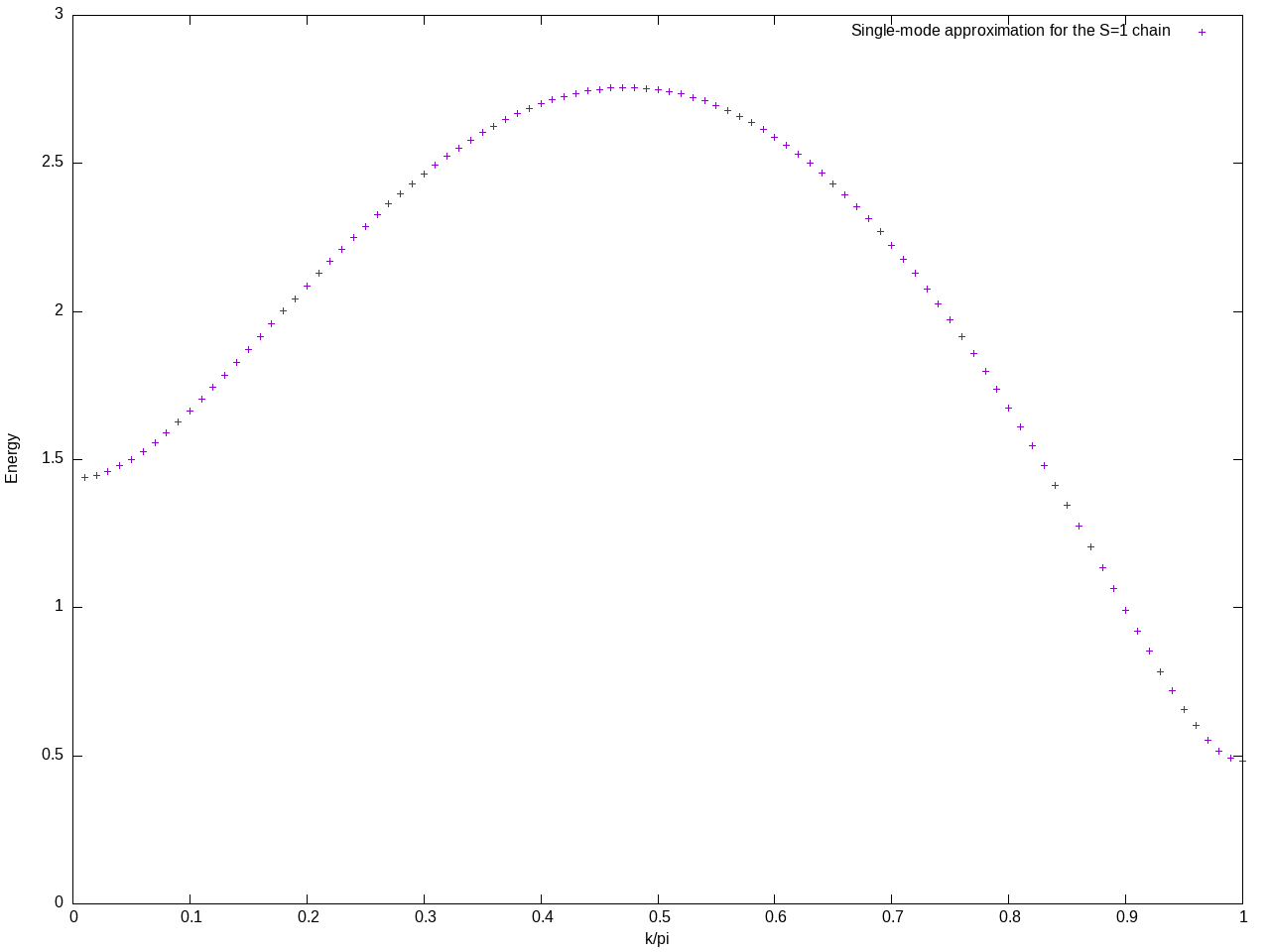 This approximation is very simple, but it gives surprisingly good results near {$k \simeq \pi$}. At {$k=\pi$} the excitation energy is the celebrated Haldane gap; more refined numerics gives an answer around 0.410479248, so our simple approximation is within around 18% of the exact value. The single-mode approximation is worse for smaller values of {$k$}, and breaks down completely around {$k = \pi/2$}, where the lowest excitation is no longer a single magnon, but a 2-particle continuum. |