• View
• Edit
• Rename
• History
• Print
• Backlinks

BinderCumulant

In this tutorial we will work through the steps to calculate the Binder Cumulant to identify a symmetry breaking phase transition.

Introduction

The Binder Cumulant is typically used with finite-size scaling. It it defined as {$$U_4 = 1 - \frac{\expect{m^4}}{3\expect{m^2}^2}$$} where {$\expect{m}$} is a {$Z_2$} order parameter (the Binder Cumulant can be obtained for other symmetry broken order parameters, but the prefactor is different).

The idea is that in the vicinity of a critical point this satisfies a scaling form {$$U_4(T,L) = {\cal U}(t L^{1/\nu})$$} where {$L$} is the system size, and {$t = T-T_c$} is some coupling constant (or temperature) with a critical point at {$t=0$}. Thus the value of {$U_4$} at the critical point {$t=0$} is independent of {$L$}, thus a plot of {$U_4$} as a function of {$T$} for several different system sizes should intersect at {$T=T_c$}.

In the thermodynamic limit, the Binder Cumulant doesn't provide anything useful -- it takes the value {$2/3$} if the order parameter is non-zero (when, in the large {$L$} limit, {$\expect{m^4} = \expect{m^2}^2$}), and 0 when the order parameter is zero (where the order parameter is Gaussian, and all cumulants vanish except for the variance, leading to {$\expect{m^4} = 3 \expect{m^2}$}). Nevertheless, for an iMPS we always have a finite correlation length, so this procedure cannot identify the critical point.

For an iMPS, the mp-imoments command calculates the moments (or cumulants) of an operator, expressed as an {$n$}-degree polynomial in the system size {$L$}, which is exact in the asymptotic large {$L$} limit. This is best expressed in terms of the cumulants per site {$\kappa_n$}. We have

{$$\expect{m}_L = \kappa_1 L$$}

which is the order parameter per site.

{$$\expect{m^2}_L = \kappa_1^2 L^2 + \kappa_2 L$$}

where {$\kappa_2$} is the variance per site (related to the susceptibility).

We also have

{$$\expect{m^4}_L = \kappa_1^4 L^4 + 6 \kappa_2 \kappa_1^2 L^3 + (4 \kappa_1 \kappa_3 + 3 \kappa_2^2)L^2 + \kappa_4 L$$}

Taking the large {$L$} limit directly gives only the leading order terms in the moments, which for the {$n$}-th moment is simply {$\expect{m}^n$}. This doesn't give anything useful, the purpose behind the Binder Cumulant is to take advantage of the higher cumulants. What we can do instead is evaluate the moments polynomial using the length scale that is available to us, namely the correlation length obtained from the transfer matrix. This gives a rather natural procedure. Note that this is only a length scale, we can in principle choose {$L = s \xi$}, where {$s$} is any fixed scaling constant. The effect of {$s$} is to change the actual value of the Binder Cumulant at the critical point (analogous to changing boundary conditions for the finite-size Binder Cumulant). We can choose {$s$} freely, to give a numerically stable fitting procedure.

Procedure

We are going to use as an example the Ising model in a transverse field. We need very few states for this, so the calculations are very fast. Firstly, we construct a lattice.

spinchain -o lattice

Now we need to construct a set of wavefunctions. For a 'real' calculation we would want to do this in a more sophisticated way, but for the Ising model it is enough to use a simple bash script, keeping from 4 to 8 states (for this example, 8 states is plenty, but less than 4 states doesn't reproduce the critical point very well).

The Ising model is surprisingly difficult to get accurate convergence, it might be necessary to run this script more than once. This is because it takes so few states, but the MPS needs to be converged to very high precision.

We now need to calculate the 4th moment of the order parameter. The order parameter is the {$z$} magnetization per site, which we could express as sum_unit(Sz(0)), or, more simply, using the lattice operator {$H_z$}. We can obtain this with, for example,

mp-imoments psi-h0.95-m7 lattice:"H_z^4"

This gives the 4th moment. We also need the 2nd moment. But these are not independent, we can obtain the 2nd moment from the 4th moment, so we don't need to do a separate calculation.

The final quantity that we need is the correlation length. We can obtain this from mp-ispectrum. The relevant correlation length corresponds to the next-leading eigenvalue.

Finally, we need to evaluate the polynomial. There are lots of ways of doing this, there is a helper program in utils/binder.cpp that takes the 4 coefficients of the 4th moment, the correlation length and the scaling factor {$s$} as parameters and calculates the Binder Cumulant. The binder.cpp program is very simple and could be scripted in many ways.

Putting all of this together, a script that calculates the Binder Cumulant for a wavefunction is

I named this program calc-binder. This assumes that the binder utility is in the path. We now need to evaluate this for each wavefunction. So we use another bash loop to write the Binder Cumulant to a file, one file for each {$m$}.

This produces a set of data files which we can plot, to produce: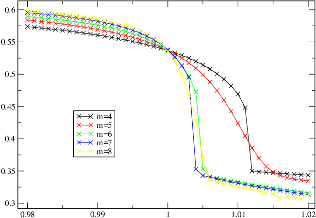

I used scaling factor {$s=5$}, chosen by trial and error.