QMBD Group Meeting 1/6/2020

This is first introduction to using the toolkit for groundstates and time evolution of finite systems, using DMRG and TEBD, using the Bose-Hubbard model. The idea for this calculation comes from https://arxiv.org/abs/1310.0281.

Preliminaries

In this tutorial, text that is in monospace font is text that will appear in the terminal. Commands that you need to type in will start with a $ sign. In some cases, the expected output will be written as well; this won't start with a $ sign. For example,

$ echo hello
hello

If you are not familiar with the command line shell, then you should try this - type 'echo hello' (then enter), and you should see 'hello' printed in response. You should also keep handy a list of basic commands - there are many available on the internet, for example

https://dev.to/awwsmm/101-bash-commands-and-tips-for-beginners-to-experts-30je#the-basics

https://www.freecodecamp.org/news/basic-linux-commands-bash-tips-you-should-know/

Getting started

Everyone is sharing the same login directory, so firstly you should make a directory for your own use, perhaps using your name.

mkdir <name>
cd <name>

Constructing the lattice file

To get started with a calculation using the Matrix Product Toolkit, the first step is to construct what is known as a lattice file. This is a file that contains a description of the lattice (i.e. the degrees of freedom at each site), as well as associated operators, such as creation/annihilation operators, symmetry transformations, and short-cut operators that we can use to help construct a Hamiltonian. The lattice file is constructed by running a program to generate it (this is a short C++ program that is in the models/ file of the source code repository. If you are curious have a look at the bosehubbard-u1-trap.cpp file to see how it works). The first example that we will look at is the Bose-Hubbard model with a harmonic trap, using {$U(1)$} particle-number symmetry. To generate the lattice file, we need to run the bosehubbard-u1-trap program. We need to supply some parameters, but if we firstly run it without then we will get a help message,

tips The shell allows using the TAB key to automatically complete commands. You can save some typing with b o s TAB u 1 - TAB and it will auto-complete to bosehubbard-u1-trap. If there is no unique completion, then TAB won't print anything -- pressing TAB again will give a list of possible completions. For example, bosehubbard TAB TAB produces a list of several variants of the bosehubbard model.

$ bosehubbard-u1-trap 
Matrix Product Toolkit version (git)
usage: bosehubbard-u1-trap [options]
Allowed options:
  --help                 show this help message
  -N [ --NumBosons ] arg Maximum number of bosons per site [default 5]
  -t [ --trapwidth ] arg Trap width [default 50]
  -o [ --out ] arg       output filename [required]

Description: U(1) Bose-Hubbard model
Author: IP McCulloch <ianmcc@physics.uq.edu.au>
Operators:
H_J        - nearest-neighbor hopping
H_U        - on-site Coulomb repulsion N*(N-1)/2
H_V        - nearest-neighbour Coulomb repulsion
H_trap     - harmonic trap, n(x)*(x-(L-1)/2)^2

Functions:
(none)

This shows that the only required option is the output filename. The other parameters we can leave as the defaults. The help message also shows some information about the Hamiltonian operators that will be constructed. In this case, there is a hopping term {$b^\dagger_i b_{i+1} + h.c.$}, local and nearest-neighbor Coulomb interactions, and a harmonic trap.

Lets generate the lattice file.

tips If you forget what the lattice file contains, use the mp-lattice-info command (or m p - l TAB to get a detailed description.

$ bosehubbard-u1-trap -o lattice

The output file is called lattice. Use the ls command to verify that it exists in the current directory.

$ ls
lattice

Groundstate wavefunction

Now we will obtain the groundstate wavefunction. The default trap width is 50 sites, so we need to construct a wavefunction with the same number of sites. For this tutorial, we will start with a random wavefunction, and use that as input for the DMRG algorithm to obtain the groundstate. To construct the random initial state, we use mp-random

$ mp-random -l lattice -u 50 -q 20 -o psi

The parameters here are -l lattice the lattice file that we previously constructed, -u 50 means construct a 50-site wavefunction (this must be the same as the trap width, otherwise we won't be able to use the trap term in the Hamiltonian), -q 20 sets the quantum numbers of the wavefunction. Since we are using {$U(1)$} particle number symmetry, this represents the number of bosons, so 20 particles in this case. Finally the -o psi is the output wavefunction.

Now we run the mp-dmrg program to use DMRG to optimize the wavefunction to be a variational approximation of the groundstate. The parameters we need are:

The input wavefunction, -w psi
The Hamiltonian. This is of the form -H lattice:expression. The expression is the Hamiltonian itself. This can be constructed from first principles (eg BH(0)*B{1} represents creating a boson at site 0, and annihilating a boson at site 1) but typically we just use the short-cut operators defined in the lattice file. So it will be some combination of H_J, H_U and H_trap. Some reasonable parameters are {$J=1$}, {$U=4$} and trap strength of {$0.05$}.
The number of states and the number of sweeps to perform. The number of states controls the accuracy of the final wavefunction, and we need to ensure that the number of optimization sweeps is sufficient for convergence. We specify both these with a parameter of the form -m 100x20, which means perform 20 sweeps with 100 basis states.

Finally, the command we will run is

$ mp-dmrg -w psi -H "lattice:H_J + 4*H_U + 0.05*H_trap" -m 100x20

Note: the quotes around the Hamiltonian are important, otherwise the shell will get confused about the spaces, * and other special characters in the Hamiltonian expression.

This should only take a few seconds to run. There will be a lot of text printed on the terminal, but near the end it will show the final energy.

Examining the groundstate

The mp-info command shows various miscellaneous bits of information about a wavefunction. The -d option can be used to show the reduced density matrix and entanglement spectrum, either at all partitions (the default) or at a specified partition with the -p option. mp-info psi -d -p 25 will show the entanglement spectrum at the half-way point of the chain. Examination of the entanglement spectrum should show that the wavefunction is symmetric about the mid-point.

tips If you forget what a wavefunction is, you can get some basic information using mp-info. This includes the most recent command that modified the wavefunction. mp-history shows the complete history of commands that modified the wavefunction.

We can also use mp-expectation to obtain various expectation values on the wavefunction. Some examples:

mp-expectation psi lattice:"N(25)" (number of particles at site 25)
mp-expectation psi lattice:"BH(20)*B(30)" (particle-hole correlation between sites 20 and 30)
mp-expectation psi lattice:"N(25)^2" (square of the local particle number)
mp-expectation psi lattice:"com(0)" (centre-of-mass)
mp-expectation psi lattice:"com(0)^2" (2nd moment of the centre-of-mass)

Time evolution

The next stage of the tutorial is to calculate the non-equilibrium real-time evolution if we quench the trap frequency. This induces breathing modes which can be probed using the 2nd moment of the centre of mass.

There are several different algorithms for the time evolution of a tensor network, which basically amount to different ways to approximate the time evolution operator {$\exp[-iHt]$}. We will use the simplest algorithm, which is known as TEBD. This utilises the Lie-Trotter-Suzuki decomposition of the Hamiltonian, to decompose it into a sequence of 2-body unitary gates. This depends on the terms in the Hamiltonian being at most nearest-neighbour. The toolkit can decompose a Hamiltonian operator into a sum of 2-body gates automatically, in most cases.

To use the mp-tebd tool there are a few parameters that we need to fix,

Choice of decomposition: there are various forms of the Lie-Trotter-Suzuki decomposition that have different error properties. We will use the default optimized4-11, which is a 4th order decomposition with error term {$\propto \Delta t^4$}.
Timestep: If the timestep is too small, then the evolution will take a long time and there is a loss of accuracy because each timestep requires basis truncations. Conversely, if the timestep is too big, then there will be errors arising from the Lie-Trotter-Suzuki decomposition (generally known as the Trotter error). For the 4th order decomposition, a timestep of 0.2 is typical.
Number of states: this controls the accuracy of the variational approximation. Because the entanglement of the wavefunction inevitably increases under time evolution, it isn't appropriate to fix the number of states to be a constant. Instead we use a cutoff eigenvalue of the reduced density matrix. In this example, {$10^{-8}$} will work OK (at least for the density - it probably isn't accurate enough to reproduce correlations accurately).
Saving the wavefunction: how often do we want to save the wavefunction? If we save the wavefunction every timestep we might run out of disk space and it will take longer to analyze, but plots will look smoother. In this example, we will save the wavefunction every 5 timesteps (so every interval of 1.0, since the timestep is {$\delta t = 0.2$}).
Total number of timesteps.
Output filename

Lets copy the wavefunction to a new name, for consistency with the time-evolved wavefunctions.

$ cp psi psi-t0.0

And construct the time evolution up to total time T=80,

$ mp-tebd -w psi-t0.0 -H lattice:"H_J + 4*H_U + 0.04*H_trap" -t 0.2 -s 5 -n 400 -d 1e-8 -o psi-t

Note that we changed the value of the trap strength from 0.05 to 0.04, which is a moderate strength quench that will excite several breathing modes. This command will produce a sequence of wavefunctions named psi-t1.0, psi-t2.0, and so on up to psi-t80.0. This will take a few minutes to run.

Properties of the time-evolution

There are many things we could do to examine the time-evolved states. The width of the distribution is a good starting point. This is the operator com(0)^2. We can evaluate this on all of the time-evolved states using a loop,

$ for t in $(seq 0 80); do mp-expectation -r psi-t$t.0 lattice:"com(0)^2" ; done

You could copy and paste this into your favourite graphing program, or save it to a file for later analysis. Note that we used the option -r to only display the real part of the expectation value. The operator com is Hermitian so in principle the expectation value is real-valued, but numerically there may be a small imaginary component of order {$\epsilon$} (machine precision).

The output should look something like: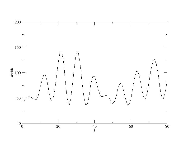

Plot of the 2nd moment of the centre of mass

which shows that there are at least two oscillation frequencies that have been excited (this shape continues to at least time 120).

Additional

Some extra things that we can calculate:

The energy and energy variance.

There is a technical detail that we didn't mention yet - the lattice file is actually designed for an infinite system; the trapping potential is actually periodic and repeats every 50 sites. The mp-dmrg program simply ignores terms in the Hamiltonian that extend beyond the finite size wavefunction. But this means there are some minor complications if we want to calculate some expectation values with mp-expectation, namely mp-expectation psi lattice:"H_J" won't work, because H_J is an infinite operator. Instead we need to use

$ mp-expectation psi lattice:"fsup(0,50, H_J + 4*H_U + 0.05*H_trap)"
9.306689016882382

Here we used the fsup operator, which projects an infinite operator to a finite operator with finite support, from sites 0 to 49. (In common with many conventions, the interval is represented as half-open, so [0,50) includes the first site, but doesn't include the last site.)

The above command will give the energy of the groundstate. We can also calculate the energy variance, {$\langle (H-E)^2 \rangle$}, via

$ mp-expectation psi lattice:"(fsup(0,50, H_J + 4*H_U + 0.05*H_trap) - 9.306689016882382)^2"
8.738852557144128e-07

This shows that the energy variance is quite small, meaning that 100 basis states is enough to get a quite accurate wavefunction. Contrary to what you might expect, the error in the energy in MPS calculations is linear in the variance, so if we repeated the calculation with an increased basis size so that the variance decreased by some factor {$K$}, then the difference between the variational energy and the exact energy will decrease by the same factor (this is strictly true only for an infinite system -- for a finite system there is also a quadratic term). Using this, it is possible to do an extrapolation to zero variance and get an estimate of the exact groundstate energy.

The energy of the time-evolved state

We can also calculate the energy of the {$t=0$} with respect to the quenched Hamiltonian,

$ mp-expectation psi lattice:"fsup(0,50, H_J + 4*H_U + 0.04*H_trap)"
5.217104818642688

In principle the energy should stay constant throughout the time evolution. Using TEBD, this will only be approximately true, because the wavefunction is projected to a smaller basis size after applying each 2-body gate. (There are more sophisticated time evolution algorithms such as TDVP that preserve unitarity exactly). If we calculate the energy of the {$t=80$} state,

$ mp-expectation psi-t80.0 lattice:"fsup(0,50, H_J + 4*H_U + 0.04*H_trap)"
5.214969684653424 -4.206191323493645e-16i

we see it has changed a bit, and there is also a numerically negligible imaginary part. So the time evolution isn't particularly accurate -- with some more computation time we could redo it with a smaller cutoff for the density matrix. (If we used a cutoff of {$10^{-10}$} then the energy is preserved to within {$10^{-4}$}, but the time evolution takes about 17 minutes rather than ~2 minutes.)

Wavefunction overlaps

We can calculate the overlap of two different wavefunctions using mp-overlap. For example,

$ mp-overlap psi-t1.0 psi-t0.0
#mp-overlap psi-t1.0 psi-t0.0
#Date: Mon, 01 Jun 2020 19:16:12 +1000
#size of wavefunction is 50 sites
#real                   #imag                   #magnitude              #argument(deg)          
0.42809318292897        -0.80803786874454       0.91443368846269        -62.085649532926

This is the expectation value {$\langle \: \psi(t=1.0) \: \vert \: \psi(t=0) \: \rangle = \langle \: \psi \: \vert \: \exp[iH] \: \vert \: \psi \: \rangle$}, where {$H$} is the quenched Hamiltonian. {$\psi$} isn't an eigenstate of the quenched Hamiltonian so we cannot simplify this expression any further, but as the quench is fairly small we might expect that we could approximate the result as {$\exp i E$} = 0.48169 - 0.87634i.

This expectation value should be time-translation-invariant, so we could also check eg {$\langle \psi(t=80.0) \: \vert \: \psi(t=79.0) \rangle$}.

$ mp-overlap psi-t80.0 psi-t79.0
#mp-overlap psi-t80.0 psi-t79.0
#Date: Mon, 01 Jun 2020 19:23:23 +1000
#size of wavefunction is 50 sites
#real                   #imag                   #magnitude              #argument(deg)          
0.42781229345049        -0.80962036510645       0.91570109425645        -62.147535109296

which is correct to just under 3 significant figures. (If we improve the accuracy of the time evolution by setting the cutoff to {$10^{-10}$}, the overlap improves accuracy to nearly 5 significant figures.}